

All Models are Wrong, but Some Are Useful
What I’d like to do in this blog article is to explore and talk about the ways we can think about growth and create models for natural growth that help us understand their underlying dynamics. The famous statistician George Box wrote, “All models are wrong, but some are useful.” Think about an architectural model of a building. There are all kinds of useful things that can be done with it and it helps a broad group of people with different backgrounds and skill sets envision and understand it. No one expects it to be functionally perfect (it may not have any truly functioning doors and windows), but it may be useful to see how lights hits it at different angles during different times of the day and different seasons of the year. The kinds of analyses might even be fairly complex and only of interest to a small set of specialists, but the physical model of the building itself can still stand as a useful depiction of the structure.
Growth Models are Poorly Expressed in the Media
In terms of understanding a complex situation like the one we’re experiencing with Covid-19, the media (and others) sometimes fall into the trap of either quickly characterizing a model without trying to understand its overall scope and purpose or narrowly latching on to a particular result without placing it in the context of the model’s assumptions and the nature of the raw data inputs into the model. A strong tendency also exists for people to criticize the “accuracy” of the model, again ignoring both the context of the assumptions and the limitations of the raw data inputs (anyone who has ever read a sports message board that discusses “stats” should know exactly the kind of behavior I’m talking about.) There are many ways to talk about models beyond their accuracy. We can talk about their sensitivity and robustness to the inclusion of different variables as well as their specificity and ability to be generalized. With regard to Covid-19, however, I just wish the discussion included a better simple model and understanding of natural growth.
When we’re building models, an important is to identify the key assumptions in the model and to have those assumptions translate directly to observable data. When models don’t have this characteristic, there is a disconnect between their fundamental insights and their usefulness. They tend to have two big problems: they are horribly complex or they come across as a tautology, that is, they express an obvious factual relationship (if we write more orders for larger amounts, our sales will increase). New product introduction models are weak when they are based on “market size and market share” assumptions in poorly defined markets or when the market share number is out of proportion to current sales. 5% of a $10 billion market might indeed be $500 million, but you necessarily have to achieve .05% market share and 0.5% market share before you can even start to think about 5%. This issue of matching the scale of assumptions and estimates in our models is particularly important when these estimates are then included in calculations. For example, we may have a decent estimate of an area’s population, but we may have a very loose assumption regarding exposures or infected people. The more assumptions and variables we add to a model, the more likely it is that the new data and/or calculations are out of scale or have low predictive power. In fact, it’s not at all unusual for variables to add noise and harm a model; even though the data may be accurate, it’s just not meaningful. The first reaction for people building models is to make them more complex, not to question their underlying structure and see if there is a better way to model the problem.
We Should Prefer Simple Models
Generally speaking, relatively simple models with understandable and meaningful assumptions are more useful than complex models with hidden processes. Significant problems often exist with accurate and timely data (particularly regarding the Covid 19 virus). One of the best strategies for dealing with incomplete and unreliable data is to keep your models fairly simple. We can build more complex models, but they’ll only be useful once we have more good data.
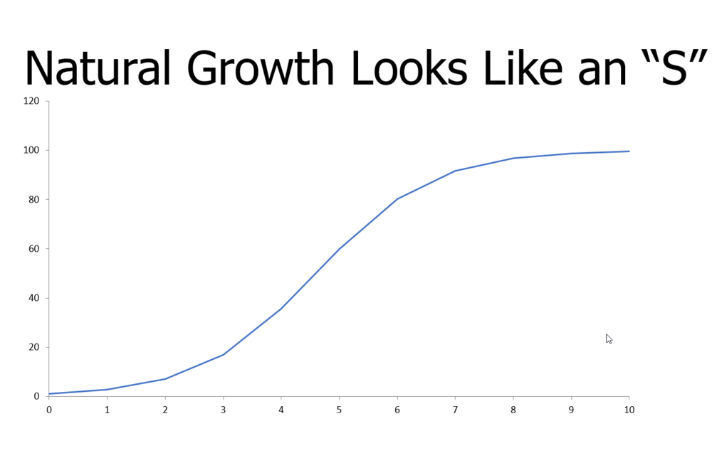
It’s possible to build a basic model of natural growth with only three variables. Most people intuitively agree that natural growth occurs in “spurts” and is highly changeable over time, but we need to start using simple non-linear mathematical models as our foundations for growth modeling.
All types of dynamic systems experience growth and decline, but almost never in a linear fashion. Whether it’s the spread of a disease, the growth of a population, the adaptation of technology, or the collapse of an eco-system, the rate of change is variable. Fortunately, we do have a relatively simple mathematical model that allows us to understand the dynamics of growth with a small number of variables, the logistic function. The logistic function is the most prominent member of the sigmoidal family of functions (s-shaped functions) and has several common expressions; we will focus on one of them.
 The Logistic Model of Growth
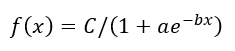
Where
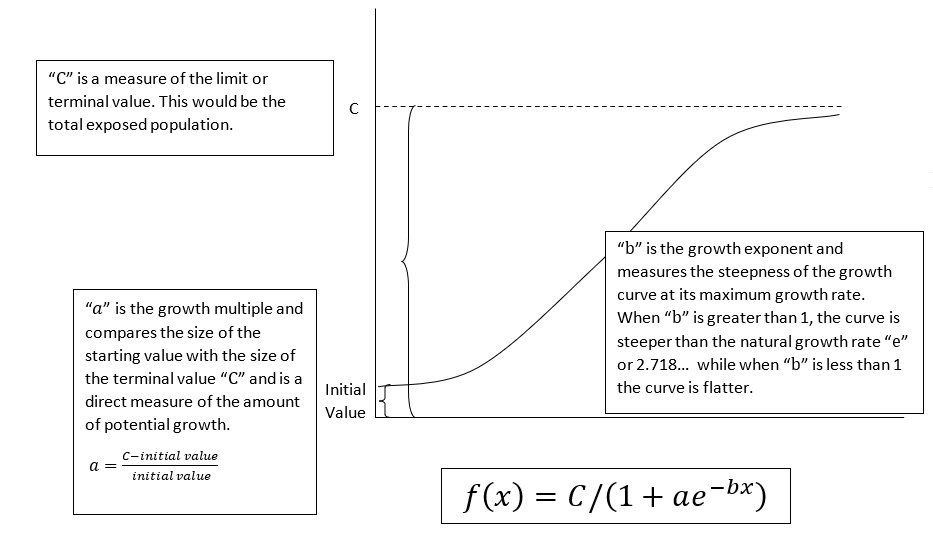
· C is the maximum value, also known as the carrying capacity or bottleneck. We can think of “C” as the growth limit.
· “a” is a proportion defined by the initial starting value compared to the limit. We can think of “” as the growth multiple.
· “b” is a modifier of the rate of change. We can think of “b” as the growth exponent.
The logistic function states that the rate of growth is proportional to the size of the population of interest and to the nearness of the size of the population of interest to its maximum amount. In other words, growth starts out slowly, accelerates, and then declines as the size of the population approaches a limiting factor. For any given scale (time period), one has to understand and estimate only three factors, the limit, the rate of change, and the initial value. This has tremendous consequences for estimation techniques. Although the equation is non-linear, it is differentiable and values can be calculated both at specific times (x axis “rate” values) and over periods of time.
The Concept Behind the Formula is Most Important
What is powerful about this model is the intuition it provides, even more so than any particular computational answers. There exist many permutations of the logistic function with different numbers of factors and different levels of simplification or complexity as any simple search on the internet will show. All of them, however, offer the same intuition.
For any given predictive model, there are critically important underlying assumptions that should be stated explicitly. Not only what is the key driver of growth during a given time period and to what degree does the growth feed on itself, but also what is the key limiting factor of growth during that same time period? What is the initial starting value at the beginning of a given time period? For scenarios where high growth is expected, what is the limiting factor and what is the period of time until the limit is reached?
Results using the logistic function are particularly sensitive to initial conditions, a common occurrence in many natural growth systems. This goes against many elements of standard practice where averages, aggregates, and other “normalizing” methods are used to smooth out results. Many models rely on detail in initial conditions, but then over-extrapolate answers. Sensitivity analysis which attempts to measure the change due to individual variables is often employed, but its power is sometimes taken away with an over reliance on averages or buried under a mound of detail where it is lost.
Living Systems Tend to Respond and React
Most systems that exhibit “complex adaptive” behavior are self-balancing. That is, they respond to pressure or incentives and the dynamics do not stay static. We’re seeing this now in our response to the Covid-19 outbreak. While some might say that “if we do nothing exponential growth will spread the virus to the entire population”. The reality is, we will respond and the spread of the disease is likely to slow after it accelerates precisely because we take responsive actions. In population theory often uses the numbers of rabbits and foxes in simple models. The number of rabbits is a function of how many predators (foxes) there are and the number of foxes is a function of how much food there is (rabbits).
Defining the Growth Limit
“C” is the maximum limit that can be achieved within the analysis period. When we are using this in the context of the spread of disease, this should be the population that has the potential to be exposed. It’s very important to match this figure with the chosen time scale on the X axis. Isolation essentially brings the limit value to the size of the household and means that we are only calculating past exposures within a limited time frame. Naturally, as the time horizon is expanded so is the chance for exposure. So as we evaluate past historic data, we can put it into a context (a time frame) that allows us to understand the underlying dynamics.
Defining the Growth Multiple
The term “a” is a measure of the starting value in comparison to the limit value “C” and can be thought of as the growth multiple. That is, it’s the proportion amount of growth that has not yet occurred. While the starting point at time “0” has a discrete value, it is better to think of “a” as a factor rather than something with a discrete value associated with it. For example, if the starting value at time “0” is fifty infected people and the growth limit “C” is fifty thousand people, then “a” has a value of nine hundred ninety – (50,000-50)/50 =990. Notice that “a” is independent of the scale of the function and allows for the comparison of different scenarios to each other. In the example above, there is a lot of growth left in the system.
The growth multiple can be thought of as a measure of the amount of growth potential within a certain period of time. A high growth multiple indicates that there is a large amount of growth built into the model while a small value of “a” indicates a smaller amount of growth. This directly avoids unlimited future growth inherent in “exponential growth” models because both the maximum value is stated explicitly “C” and because the relationship between the starting value and the maximum value is stated explicitly in the growth multiple “a”.
The logistic function is quite sensitive to the size of the initial value. When the initial value is high compared to the limiting value “C”, the model responds with fast growth. The rate of growth at a particular point in time is a function of the amount of infected people in the previous period. While straight-line growth is best suited to situations with a high degree of aggregation and averaging, the logistic function works best in situations of high independence and non-aggregation.
Defining the Growth Exponent
How to estimate the growth exponential “b” may not be immediately apparent on an intuitive basis. We can consider “b” to be the growth exponent. If “b” is equal to 1, then the function acts according the natural logarithmic function “e”. Think of this as natural, organic growth. If “b” is greater than 1, then growth is more recursive, steeper than natural growth, and is compressed into a shorter period of time. Discrete amounts of growth are low in the beginning of the chosen period, highest in the middle, and low in the end. Likewise, if “b” is less than one but greater than zero, the growth is slower and the “S” is more horizontal and less steep. Rates of growth are more consistent across the chosen time frame. (If “b” is negative, the “S” is inverted and the function shows accelerating decline rather than growth.) Computing an actual value of “b” is less important than examining the feedback loop in the rate of growth and considering the possibility of a “virtuous” cycle in which accelerating rates of growth beget even stronger rates of growth for period of time. Exceptionally low values of “b” will approximate a traditional, straight line growth curve. We can also think of “b” as a measure of recursiveness showing how much growth is due to exogenous factors and how much growth is dependent on endogenous factors. Alternatively,
it can be thought of as a measure of the persistence of growth.
While additional terms can be added to the equation to shift the skewness and kurtosis of the curve, they add a lot of mathematical complexity. For the purposes of projections and estimates, most adjustments to the model should be made by changing the time period over which a given estimate is made.
Logistic Function Growth
The real benefit of using logistic growth models comes from asking a small number of good questions about the assumptions.
· What is the time period in which we are considering exposure? (time period on the X axis)
· What is total exposed population? ( or the growth limit)
· What is the proportional relationship between the starting number of infected people and the total exposed population? ( or the growth multiple)
· And finally, what is the “contagiousness” of the disease? ( or the growth exponent)
If we believe that the situation is highly dynamic and that our factors are changing, all we need to do is to choose a specific, discrete time period and check our assumed values. This becomes a simpler, and more structured way of evaluating contagion and disease spread rather than trying to report a “growth rate” (which is continually changing across time) or to invoke an ill-defined notion of “exponential growth” which excludes the natural balancing dynamic that typically occurs in complex adaptive systems.
The logistic growth formula has direct parallels in business valuation techniques (it’s particularly useful in modeling high growth technology firms where more traditional valuation models of growth like the terminal value model break down), population growth in ecosystems, and economic growth models. It’s extremely easy to code for a logistic growth model or even build a simple model in excel. You can draw your growth curve graph, make changes to your assumptions and see it play out directly. If anyone wants a simple excel spreadsheet with the formulas already in it, just send me a request to tvlamis@vlamis.com and I’ll send it along to you.